Alignment and Dynamic Programming

For this lab we will focus on protein similarity and in the process learn about a very powerful and versatile programming technique, namely “Dynamic Programming”.

As you have learned previously, proteins are structured in several levels. Here we will examine, similarity at the primary level ie we will compare 2 the amino-acid sequences. An amino-acid sequence contains all the information required to determine the 3D structure of the protein in a given environment thus by focusing there we don't have to worry about environmental factors. Conveniently, it is also easier to deal with simple strings than 3D structures.

Identifying protein similarity is a very important task of modern biology. It is important both for the study of molecular biology, because it allows us to categorize and abstract and also for the study of evolutionary biology because it allows us to identify homolog proteins across species.

In this lab, we will first learn about Dot Plots and easy visual method to identify regions of similarity. Then we will learn about Dynamic Programming and we will see how we can apply it to evaluate the Levenshtein similarity of two sequences.

Dot Plot

Given two sequences \(x_i, y_j\) we construct a matrix \(S_{i,j}\) in the following way:

$$ S_{i,j} = \begin{cases} 1 & x_i = y_j \ 0 & x_i \neq y_i \end{cases} $$

Below is an example for the strings X = "THISSTRING" and Y = "THISISASTRING".

dotmatrix <- function(X, Y) {
    X <- strsplit(X, "")[[1]]  # turn the string into a vector
    Y <- strsplit(Y, "")[[1]]
    S <- sapply(X, function(x) x == Y)  # Check every letter of X with Y
    S <- S + 0L  # turn logical matrix into integer
    rownames(S) <- Y
    return(S)
}

S <- dotmatrix("THISSTRING", "THISISASTRING")
plot_tableau(S, main = "Dot Plot", col = c("#619CFF", "#F8766D"), txt=FALSE)

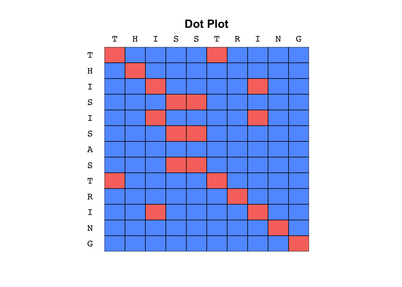
Key points to notice:

• The main point of interest are diagonal lines
  • Straight diagonals indicate consecutive matches
  • Breaks in diagonals indicate local mismatches
  • Vertical shifts indicate deletions in X
  • Horizontal shifts indicate insertions in X
• Dot plots are useful to quickly recognize repeats in the 2 sequences (or in single sequence when compared with itself)
• It's a “visual” method
• It's sensitive to noise.

The most widely used software for Dot-plots is Dotter now part of Seqtools

Noise Filter

We can deal with noise the same way we deal with it in any image processing task namely, apply a “kernel” smoother. A kernel smoother (in its simplest form) is a window focused and a cell making a decision about the cell's value. Since we are dealing with binary matrices, we are interested whether the cell is active (1) or not (0). The kernel-windows has size W which correspond to the number of neighboring cells involved and is associated with a decision process. Here the decision process is very simple, we just count the number of active neighbors and if it's above a predefined threshold L we call the cell active otherwise not. Finally, since we are only interested in diagonal lines, the shape of the kernel is diagonal, meaning that horizontal of vertical cell neighbors do not contribute to the decision. Below is a simple implementation of these ideas:

dotplot_filter <- function(S, W=3, L=2){
    # S is the dotplot matrix we wish to de-noise
    # W, L are the size of the kernel and the threshold repsectively.
    # They have default values so the user does not need to specify them everytime.
    
    if (L > W) return(matrix(0, nrow = nrow(S), ncol = ncol(S)))
    if (W %% 2 == 0) stop("W must be odd")
    Wflank <- W %/% 2  # how many cells back and font to look for W=3 -> Wflank=1 (1 back and 1 front)
    
    Sclean <- S  # Copy S
    Sclean[] <- 0  # Fill with 0
    for (i in 1:nrow(S)) {
        for (j in 1:ncol(S)) {
            # for every cell i,j
            for (w in -Wflank:Wflank) {
                # move along the diagonal with w
                # tryCatch = when the index is not there don't raise Error just continue
                tryCatch({Sclean[i,j] <- Sclean[i,j] + S[i+w,j+w]}, error = function(e) e)
            }
        }
    }
    return((Sclean >= L) + 0)
}

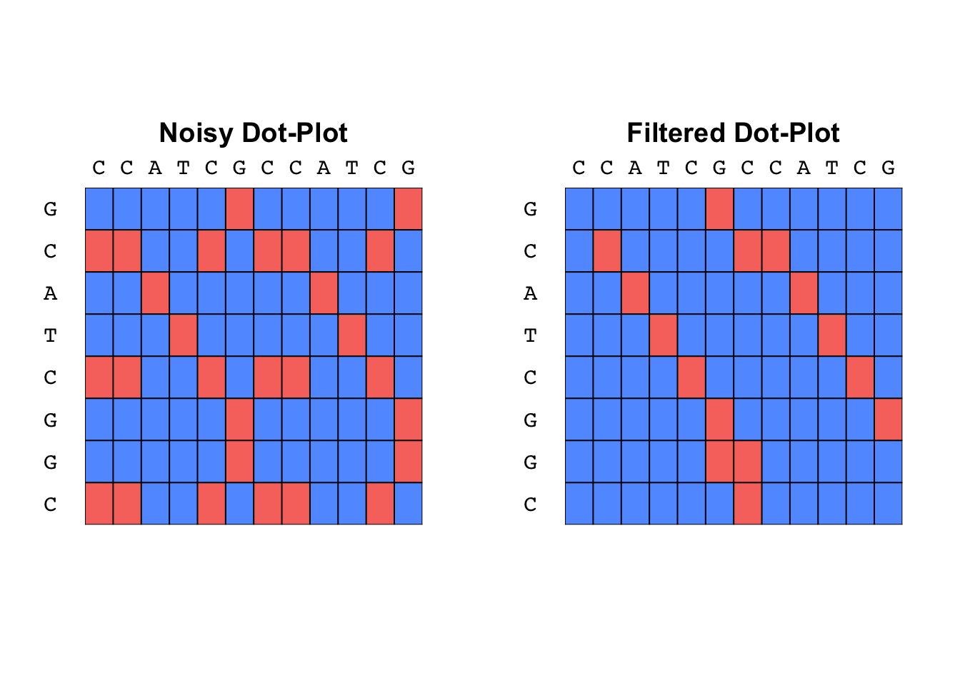
noisy_S <- dotmatrix("CCATCGCCATCG", "GCATCGGC")
quiet_S <- dotplot_filter(noisy_S)
par(mfrow=c(1,2))  # combine 2 plots
plot_tableau(noisy_S, col = c("#619CFF", "#F8766D"), txt = FALSE)
title("Noisy Dot-Plot")
plot_tableau(quiet_S, col = c("#619CFF", "#F8766D"), txt = FALSE)
title("Filtered Dot-Plot")

Distance Metrics

The notion of similarity is usually defined in terms of a distance metric. In practice it's the inverse of a particular distance metric, although “inverse” may mean different things depending on the distance metric used.

Hamming Distance

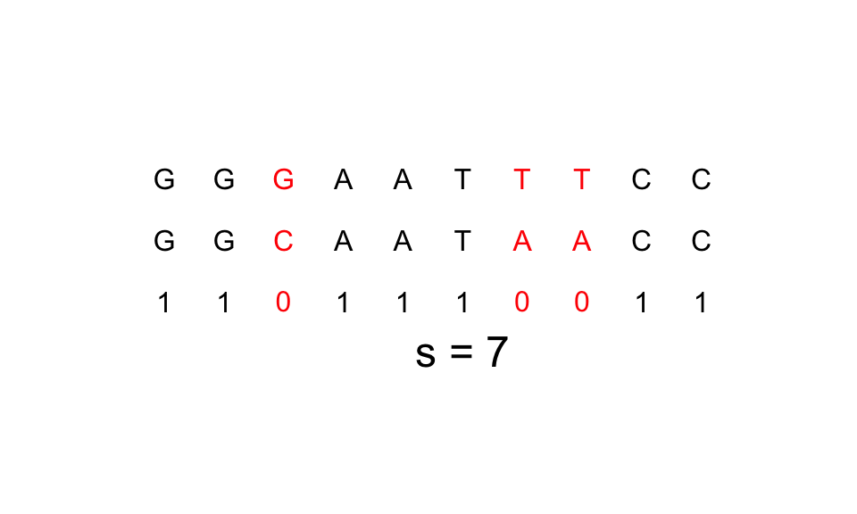
A very popular distance metric for strings is the Hamming distance. The hamming distance is defined for two equally long strings as the number of corresponding letters that don't match. So inversely, hamming similarity is the number of corresponding letters that do match.

An example with X="GGGAATTTCC" and Y="GGCAATAACC" is shown below:

However, the hamming distance is not appropriate for comparing proteins because:

• it is not straight forward how it can be expanded to unequal long strings
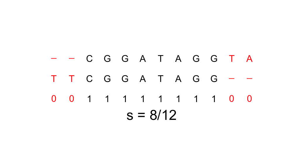
• it is not close to our “intuitive” understanding of “similar” with respect to proteins. See the following example for X="CGGATAGGTA" and Y="TTCGGATAGG":

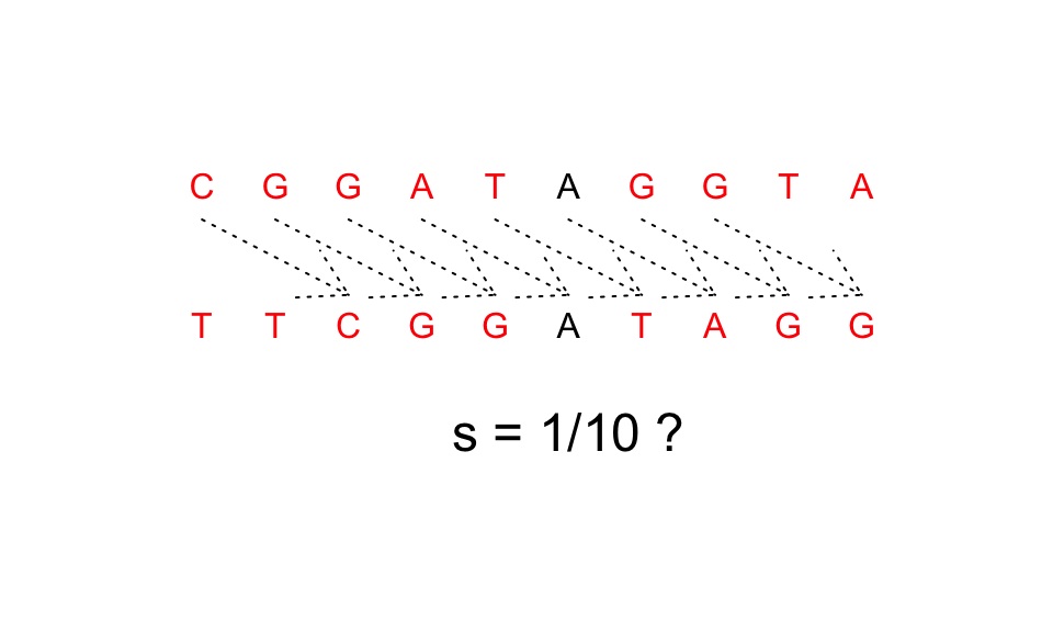
For this last example, hamming distance considers the 2 strings completely different but intuitively we fill that they are the same string moved two spots.

Levenshtein Distance

From Wikipedia:

The Levenshtein distance between two words is the minimum number of single-character edits (i.e. insertions, deletions or substitutions) required to change one word into the other.

This corresponds better with our intuition for protein similarity and for the last example it yields:

Because it requires 4 changes (2 deletions and 2 insertions) to make the strings match.

Dynamic Programming

From Wikipedia

Dynamic programming is a method for solving a complex problem by breaking it down into a collection of simpler subproblems, solving each of those subproblems just once, and storing their solutions. The next time the same subproblem occurs, instead of recomputing its solution, one simply looks up the previously computed solution, thereby saving computation time at the expense of a (hopefully) modest expenditure in storage space.

It is better understood through an example

Maximum Independent Set of a Path graph

Given a finite arithmetic sequence of positive integers, find the sub-sequence with the maximum sum without selecting 2 adjacent elements. Eg: A = [5, 2, 8, 6, 3, 6, 7, 9]

If we follow the definition:

Dynamic programming is a method for solving a complex problem by breaking it down into a collection of simpler subproblems,

We need to understand what “simpler” means in this problem. The most natural measure of complexity is the size of the input. Here we have a sequence of 8 numbers which we are not sure how to solve but we are very confident that we could find the solution to sequences of length 0, 1 or even 2. So now the question becomes: how can me construct a solution to bigger problems given the solution to the small ones?

To answer this, we need one key observation about the optimal sub-sequence. We need to understand how the solution changes as the problem get smaller. So if we peel-off the last element of our sequence (here 9) how does the optimal solution change?

Let's denote the original sequence \(A_8\) because it has all 8 elements and its optimal sub-sequence \(S_8\). Then there are only 2 possibilities:

1. \(a_8 \notin S_8 \Rightarrow S_8 = S_7\) (Think why!)
2. \(a_8 \in S_8 \Rightarrow S_8 = S_6 + a_8\) (Think why!)

So if someone gave us the answers \(S_6\) and \(S_7\) we could easily find the solution to \(S_8\) as: $$S_8 = \max(S_7, S_6 + a_8)$$ But \(S_6\) and \(S_7\) are the solution to \(A_6\) and \(A_7\) 2 “new” sequences! So we can apply our logic again and again until we reach \(A_1\) and \(A_2\) where the answer is easy.

So in general we can write for any sequence of \(A_n\) of \(n\) letters with elements \(a_n\):

$$S_i = \begin{cases}\max(S_{i-1}, S_{i-i} + a_i) & i > 1 \\ a_1 & i = 1 \\ 0 & i = 0 \end{cases}$$

and the sum of the optimal sub-sequence would be \(S_n\).

Below is the code for such a function and the original example

opt_subseq_sums <- function(A) {
    # given the sequence A this function returns a vector with all the optimal
    # subsequences S_i of A_i (the first i elements of A). The last element 
    # is the sum of the optimal subsequence of A.
    
    S <- rep(0, length(A) + 2)  # a vector of zeros
    # we added 2 extra elements to avoid the special cases of S[1], S[2]
    
    if (length(A) == 0) return(0)
    for (i in 1:length(A)) {
        # we add 2 at every S index because of the 2 artificial entries
        S[i+2] <- max(S[i+1], S[i] + A[i])
    }
    return(S[3:length(S)])  # we don't return the first two entries (0,0)
}

A <- c(5, 2, 8, 6, 3, 6, 7, 9)
S <- opt_subseq_sums(A)
cat(S)

## 5 5 13 13 16 19 23 28

As you may have notice, S only contains the sums of the optimal sub-sequences, not the sub-sequences themselves. If we are interested in them (and we are!) we can reconstruct them. One solution is to rewrite the function and keep track of our movement. But if that isn't possible (say you use someone else's code) then you can easily reconstruct afterwards. Below is the code to do so and we apply it to the S we computed before

reconstruct_subseq <- function(A, S) {
    # Given the sequence and the matrix S of optimal subsequences, this function
    # reconstruct the optimal subsequence
    
    subA <- c()  # the optimal subsequent
    i <- length(S)  # we start from the end and work our way back
    while (i > 1) {
        if (S[i] == S[i-1]) {
            # we here from the previous cell so the current cell is not added
            i <- i - 1  # move to previous cell
        }
        else {
            # we added the current value to get here
            subA <- c(A[i], subA)  # add the element to subsequence
            i <- i - 2  # move 2 cells back
        }
    }
    
    # there are 2 cases now (we stop to avoid error at S[i-1])
    # 1: jumped from the 2nd position to 0 so there is nothing to do or
    # 2: we reached 1 so we have to add the last element as well
    if (i == 1) subA <- c(A[1], subA)
    
    return(subA)
}

A <- reconstruct_subseq(A, S)
cat(A)

## 5 8 6 9

Compute Levenshtein Similarity

The same logic that we used to solve the optimal sub-sequence problem applies in solving the optimal alignment problem. We have to:

1. Recognize the “standard” form of the problem
2. Recognize the “size” of the problem
3. Imagine how we could construct the optimal solution if we decrement the size.
4. Apply the same scheme to the smaller problems until we reach a tractable problem that we can solve fast.

In the following section we will follow these steps.

The Standard form of the problem.

A formal description of the problem is the following:

Given two strings \(X=x_1x_2...x_m\) and \(Y=y_1y_2...y_n\) with \(x_i, y_j \in \Sigma\) where \(\Sigma = \{A, C, ... Y\}\) the alphabet of aminoacids and a gain function \(G: (x_i, y_j) \rightarrow \mathbb{R}\). Find the alignment of \(X, Y\) that yields the greatest gain.

The gain function, takes as input 2 letters from the alphabet and returns a number. So when we ask for the “alignment that yields the greatest gain” we simply have to extend the definition to strings. For 2 strings of equal length, we can simply write:

$$ G(X, Y) = \sum_iG(x_i, y_i)$$

For unequal string the formula is the same, we just have to extend the shorter one with gaps. For now we assume that \(G\) also scores gaps with letters but later we will see that gaps are a special case.

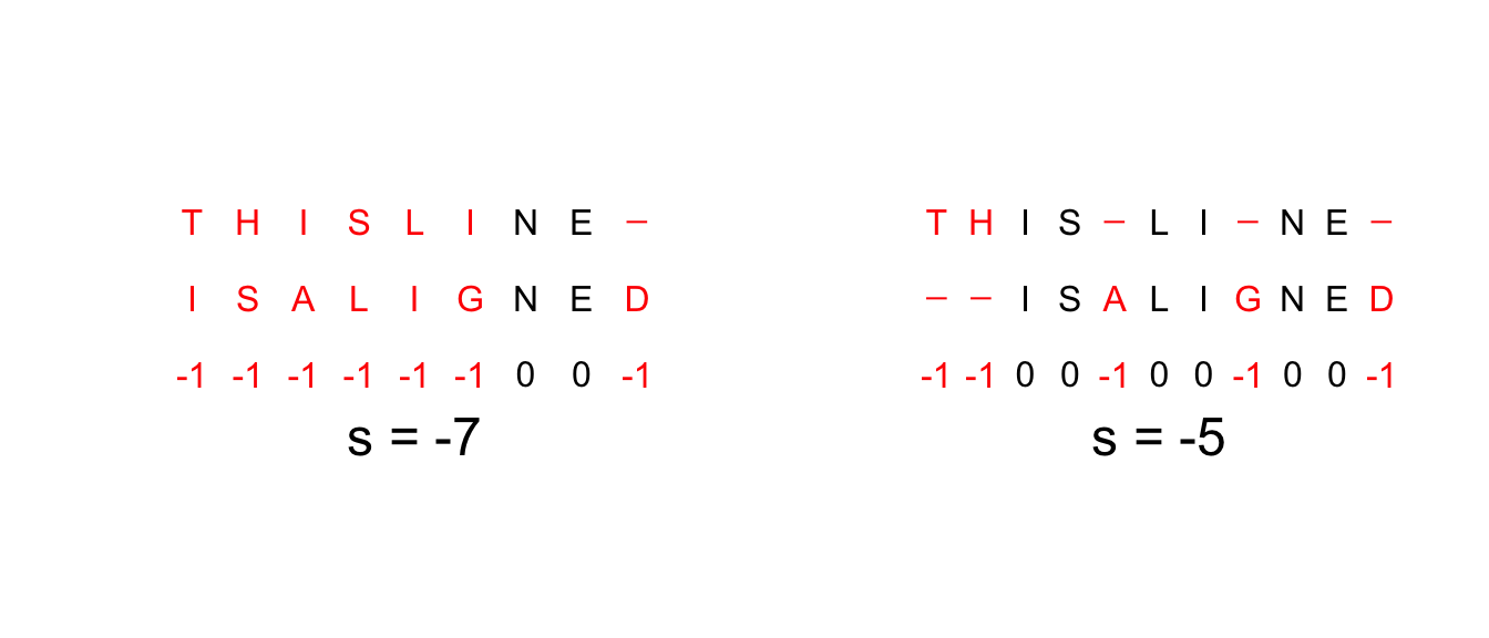
So for example, given the strings X = "THISLINE" and Y = "ISALIGNED" and gain function G <- function(x, y) -(x != y) we can easily compute the total gain by matching their letters one by one and adding gaps at the end. But this is not their distance because there is a better alignment that yields a better result (see below).

The size of the problem.

The first key step in solving all dynamic programming problem is to understand what is the size of the problem. While before it was fairly obvious, we had one sequence of specific length, here is not so because there are 2 strings and they may even be unequal. Moreover, the final alignment may have lengthen one or both of them.

However, if we shift our attention from the given strings to the final, optimally aligned, strings the problem simplifies greatly. In the optimal alignment, we would have 2 new strings of equal length composed from letters from the initial strings plus gaps. So the situation would look like this:

$$ \begin{aligned} \hat{X} &= \hat{x}_1\hat{x}_2...\hat{x}_k & \hat{x} &\in \{x_1,...,x_m, \_\}\\ \hat{Y} &= \hat{y}_1\hat{y}_2...\hat{y}_k &\hat{y} &\in \{y_1,...,y_n, \_\} \\ \end{aligned} $$

and the maximum gain would be \(G(\hat{X}, \hat{Y})\)

Thus we have a concrete size to work with, namely \(k\) the length of the final alignment! Now all we have to do is focus on the sub-problem structure and derive how we can construct the optimal solution from them.

Structure of Subproblems

As before, the key is to focus on the last elements, namely \((\hat{x}_k, \hat{y}_k)\). There are 3 possible alignment for these elements:

$$ \begin{aligned} \hat{x}_k &= x_m & \hat{y}_k &= y_n \\ \hat{x}_k &= x_m & \hat{y}_k &= \_ \\ \hat{x}_k &= \_ & \hat{y}_k &= y_n \end{aligned} $$

And for each case we have a new pair of strings to align \((X', Y')\) which as a pair are smaller! These are for each situation:

$$ \begin{aligned} X' &= x_1...x_{m-1} & Y' &= y_1...y_{n-1} \\ X' &= x_1...x_{m-1} & Y' &= Y \\ X' &= X & Y' &= y_1...y_{n-1} \end{aligned} $$

So now if someone handed us the solutions for each of these pairs \(S_{X',Y'}, S_{X',Y}, S_{X,Y'}\), we could construct the solution to the original pair \(S_{X,Y}\) by merely comparing all the possibilities and choosing the best:

$$ S_{X,Y} = \max\begin{cases} S_{X’,Y’} &+& G(x_m, y_n) \ S_{X’,Y} &+& G(x_m, _) \ S_{X,Y’} &+& G(_,y_n) \end{cases} $$

For which we can apply the same trick! Until when? Until one of the 2 original strings run out! Because, we all know that the only way to align an empty string with any other string is by filling it with gaps, ie all the letters must be inserted/deleted!

Global Alignment - Needleman-Wunsch Algorithm

Below is the code for the solving the optimal alignment problem. It's a (as much as possible) faithful implementation of the described mathematical model.

align <- function(X, Y, G, gap) {
    ## Prepare data
    # get sizes
    n <- nchar(X)
    m <- nchar(Y)
    # Turn strings into vectors
    X <- unlist(strsplit(X, ""))
    Y <- unlist(strsplit(Y, ""))
    
    # Initialize the Matrix S
    S <- matrix(0, nrow = n+1, ncol = m+1) # full of 0, n+1 and m+1 to accound for S_{0,0}
    rownames(S) <- c("_", X)  # all the letters of X plus the "empty" string
    colnames(S) <- c("_", Y)
    # Initialize 1st row/col
    S[,1] <- 0:n * gap  # make a vector from 0 to n and multiply it with gap
    S[1,] <- 0:m * gap
    
    ## Main loop
    for (i in 1:n) {  # for all substrings of X
        for (j in 1:m) {  # for all substrings of Y
            Match <- S[i,j] + G[X[i], Y[j]]
            Insertion <- S[i, j+1] + gap  # Gap at Y 
            Deletion <- S[i+1, j] + gap   # Gap at X
            S[i+1,j+1] <- max(Match, Insertion, Deletion)
        }
    }
    return(S)
}

Notice that:

• To construct S[i+1, j+1] we only use element that are before it.
• The gain function G is a matrix (inputs take values from finite field)
• gap is a separate argument not encode by G and constant.

Below is the solution to the example given before:

X <- "THISLINE"
Y <- "ISALIGNED"
# get amino-acid letters
Aminos <- read.csv("Amino-acids.csv", stringsAsFactors = FALSE)[["letters"]]
n <- length(Aminos)
G <- diag(1, n, n) - 1  # simple cost function
colnames(G) <- rownames(G) <- Aminos
print(G)

##    A  R  N  D  B  C  E  Q  Z  G  H  I  L  K  M  F  P  S  T  W  Y  V
## A  0 -1 -1 -1 -1 -1 -1 -1 -1 -1 -1 -1 -1 -1 -1 -1 -1 -1 -1 -1 -1 -1
## R -1  0 -1 -1 -1 -1 -1 -1 -1 -1 -1 -1 -1 -1 -1 -1 -1 -1 -1 -1 -1 -1
## N -1 -1  0 -1 -1 -1 -1 -1 -1 -1 -1 -1 -1 -1 -1 -1 -1 -1 -1 -1 -1 -1
## D -1 -1 -1  0 -1 -1 -1 -1 -1 -1 -1 -1 -1 -1 -1 -1 -1 -1 -1 -1 -1 -1
## B -1 -1 -1 -1  0 -1 -1 -1 -1 -1 -1 -1 -1 -1 -1 -1 -1 -1 -1 -1 -1 -1
## C -1 -1 -1 -1 -1  0 -1 -1 -1 -1 -1 -1 -1 -1 -1 -1 -1 -1 -1 -1 -1 -1
## E -1 -1 -1 -1 -1 -1  0 -1 -1 -1 -1 -1 -1 -1 -1 -1 -1 -1 -1 -1 -1 -1
## Q -1 -1 -1 -1 -1 -1 -1  0 -1 -1 -1 -1 -1 -1 -1 -1 -1 -1 -1 -1 -1 -1
## Z -1 -1 -1 -1 -1 -1 -1 -1  0 -1 -1 -1 -1 -1 -1 -1 -1 -1 -1 -1 -1 -1
## G -1 -1 -1 -1 -1 -1 -1 -1 -1  0 -1 -1 -1 -1 -1 -1 -1 -1 -1 -1 -1 -1
## H -1 -1 -1 -1 -1 -1 -1 -1 -1 -1  0 -1 -1 -1 -1 -1 -1 -1 -1 -1 -1 -1
## I -1 -1 -1 -1 -1 -1 -1 -1 -1 -1 -1  0 -1 -1 -1 -1 -1 -1 -1 -1 -1 -1
## L -1 -1 -1 -1 -1 -1 -1 -1 -1 -1 -1 -1  0 -1 -1 -1 -1 -1 -1 -1 -1 -1
## K -1 -1 -1 -1 -1 -1 -1 -1 -1 -1 -1 -1 -1  0 -1 -1 -1 -1 -1 -1 -1 -1
## M -1 -1 -1 -1 -1 -1 -1 -1 -1 -1 -1 -1 -1 -1  0 -1 -1 -1 -1 -1 -1 -1
## F -1 -1 -1 -1 -1 -1 -1 -1 -1 -1 -1 -1 -1 -1 -1  0 -1 -1 -1 -1 -1 -1
## P -1 -1 -1 -1 -1 -1 -1 -1 -1 -1 -1 -1 -1 -1 -1 -1  0 -1 -1 -1 -1 -1
## S -1 -1 -1 -1 -1 -1 -1 -1 -1 -1 -1 -1 -1 -1 -1 -1 -1  0 -1 -1 -1 -1
## T -1 -1 -1 -1 -1 -1 -1 -1 -1 -1 -1 -1 -1 -1 -1 -1 -1 -1  0 -1 -1 -1
## W -1 -1 -1 -1 -1 -1 -1 -1 -1 -1 -1 -1 -1 -1 -1 -1 -1 -1 -1  0 -1 -1
## Y -1 -1 -1 -1 -1 -1 -1 -1 -1 -1 -1 -1 -1 -1 -1 -1 -1 -1 -1 -1  0 -1
## V -1 -1 -1 -1 -1 -1 -1 -1 -1 -1 -1 -1 -1 -1 -1 -1 -1 -1 -1 -1 -1  0

S <- align("THISLINE", "ISALIGNED", G, gap = -1)
plot_tableau(S)  # custom function

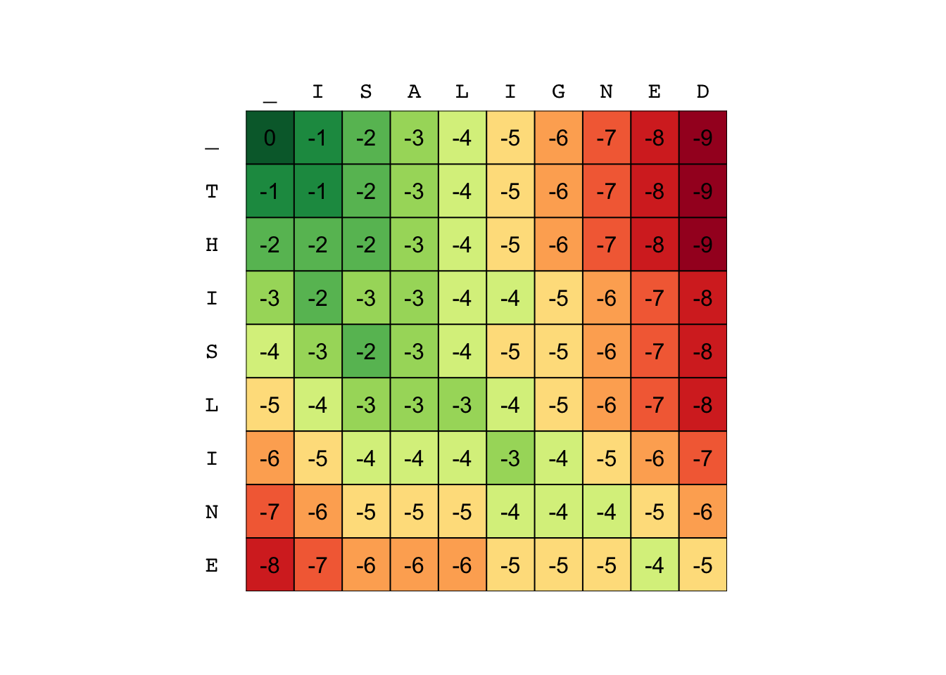
This matrix contains the solution to every combination of sub-strings from “THISLINE” and “ISALIGNED”. The first row for example is the empty string with all the sub-strings of “ISALIGNED” and S[5,3] is the solution to aligning “THIS” with “IS”). So the solution is at the bottom right corner (-5)

But which alignment yields this score?

Alignment Reconstruction

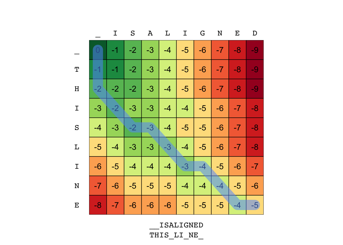
To answer that we need to roll-back the steps and starting from the bottom right go all the way up to the top left. For every move we fill in the alignment accordingly:

• Move left: the letter of the top string changes but on the left is the same so we add a “_” on \(X\) and the column letter on \(Y\)
• Move up: the letter on the left changes but on top is the same. We add “_” on the \(Y\) and the row letter on \(Y\)
• Move diagonally: both row and column change so we add the row letter on \(X\) and the column on \(Y\).

Ideally, you would keep track of your movements while constructing the matrix. We will do that in the next section. If you only have the matrix S and the gain function G you can easily trace-back the path. Below is a function that implements this logic:

backtrack <- function(S, G, gap) {
    ## Prepare Data
    # Strings to align
    X <- rownames(S)
    Y <- colnames(S)

    ## Initialize    
    Ax <- Ay <- NULL  # Empty vectors to hold letters from X and Y
    # Start at bottom right corner
    i <- nrow(S)
    j <- ncol(S)
    # To keep track of the path for ploting
    I <- c(i); J <- c(j)
    
    ## Main loop
    while (i > 1 & j > 1) {
        if ( S[i, j] == (S[i-1, j-1] + G[X[i], Y[j]]) ) {
            # it moved diagonally
            Ax <- c(X[i], Ax)
            Ay <- c(Y[j], Ay)
            i <- i - 1
            j <- j - 1
        } else if ( S[i, j] == (S[i, j-1] + gap) ){
            # it moved horizontally
            Ax <- c("_", Ax)
            Ay <- c(Y[j], Ay)
            j <- j - 1
        } else {  # S[i,j] == S[i-1, j] + gap
            # it moved vertically
            Ax <- c(X[i], Ax)
            Ay <- c("_", Ay)
            i <- i - 1
        }
        # to plot the path later
        I <- c(I, i)
        J <- c(J, j)
    }
    
    # We are not done! It may have ended in top-row or left-column (i or j == 1?)
    # We must fill until top-left cell
    if (i == 1 && j > 1){
        # X is exchausted -> fill up Y and complete with _
        Ax <- c(rep("_", j-1), Ax)
        Ay <- c(Y[2:j], Ay)
        I <- c(I, rep(1L, j-1))
        J <- c(J, (j-1):1)
    } else if (i > 1 && j == 1) {
        # Y is exchausted -> fill up X and complete with _
        Ax <- c(X[2:i], Ax)
        Ay <- c(rep("_", i-1), Ay)
        I <- c(I, (i-1):1)
        J <- c(J, rep(1L, i-1))
    }
    
    return(list(X = Ax, Y = Ay, path = list(x = I, y = J)))
}

Now you can see what the backtrack function returns and if we pass this info to plot_tableau you get a more informative figure.

al <- backtrack(S, G, gap = -1)
print(al)

## $X
##  [1] "T" "H" "I" "S" "_" "L" "I" "_" "N" "E" "_"
## 
## $Y
##  [1] "_" "_" "I" "S" "A" "L" "I" "G" "N" "E" "D"
## 
## $path
## $path$x
##  [1] 9 9 8 7 7 6 5 5 4 3 2 1
## 
## $path$y
##  [1] 10  9  8  7  6  5  4  3  2  1  1  1

plot_tableau(S, al)  # custom function

Built-in Backtrack

To keep track of the path as we fill the matrix S we have to make some small changes to the align function. In particular, we have to store for each cell the location of the previous cell. Because we need a single value for each cell we will use the linear indexing scheme instead of the standard subscript indexing. In this scheme, position 1 corresponds to the cell [1,1] and as we increment the position (2, 3, ...) we move down across the rows (first dimension) until we run out of rows and then we move to the next column.

Below is the same align function re-implemented to keep track of the each cell predecessor. The function sub2ind is used to transform the subscripts [i,j] to a single index ind.

align <- function(X, Y, G, gap) {
    ## Prepare Input  
    n <- nchar(X); 
    m <- nchar(Y) 
    X <- unlist(strsplit(X, ""))
    Y <- unlist(strsplit(Y, ""))
    # function to transform subscripts to linear index
    sub2ind <- function(r, c) (c-1) * nrow(S) + r
    
    ## Initialize Matrices
    S <- matrix(0, nrow = n+1, ncol = m+1)
    rownames(S) <- c("_", X)
    colnames(S) <- c("_", Y)
    S[,1] <- 0:n * gap
    S[1,] <- 0:m * gap
    
    # The matrix to hold the "predecesors"
    P <- S
    P[,1] <- 0:n
    P[1,2:ncol(S)] <- sub2ind(1, 1:m)  # transform index to linear

    # Main loop
    for (i in 1:n) {
        for (j in 1:m) {
            Candidates <- c(
                Match = S[i,j] + G[X[i], Y[j]],
                Insertion = S[i, j+1] + gap,
                Deletion = S[i+1, j] + gap
            )
            # For each candidate the coordinates (r, c) of the predecesor are:
            predecesors <- list(r = c(i, i, i+1), 
                                c = c(j, j+1, j)) 
            
            # Find the optimal!
            imax <- which.max(Candidates)  # index of maximum value
            S[i+1, j+1] <- Candidates[imax]
            P[i+1, j+1] <- sub2ind(predecesors$r[imax], predecesors$c[imax])
            
        }
    }
    return(list(S = S, P = P))  # notice that now we are returning 2 matrices!
}

And the backtrack now simplifies

backtrack <- function(S, P) {
    # Start at bottom right corner
    start <- length(P)  # the last position
    
    # Reconstruct the path
    path <- NULL
    while (start > 0) {
        path <- c(start, path)  # prepend start
        start <- P[start]  # move to the next position in P
    }
    I <- ((path - 1) %% nrow(P)) + 1  # indices of Rows
    J <- floor((path - 1) / nrow(P)) + 1  # indices of Columns
    
    # Alignment
    reconstruct <- function(steps, letters) {
        A <- c(FALSE, diff(steps) > 0)
        A[A] <- steps[A]
        A[A == 0] <- 1
        return(letters[A[-1]])
    }
    Ax <- reconstruct(I, rownames(P))  # aligned version of x
    Ay <- reconstruct(J, colnames(P))  # aligned version of y
    
    return(list(X = paste0(Ax), Y = paste0(Ay), path = list(x = I, y = J)))
}

The reconstruct function takes advantage of the fact that when following the path along one dimension, a letter is used only when the index decreases by one. Understanding all the details is not very important but you are welcome to investigate.

Because we are going to see many variation of the alignment algorithm we would have to change the staring point for backtracking often start. So we will split the backtrack like this:

backtrack_main <- function(P, start) {
    # Reconstruct the path
    path <- NULL
    while (start > 0) {
        path <- c(start, path)  # prepend start
        start <- P[start]  # move to the next position in P
    }
    I <- ((path - 1) %% nrow(P)) + 1  # indices of Rows
    J <- floor((path - 1) / nrow(P)) + 1  # indices of Columns
    
    # Alignment
    reconstruct <- function(steps, letters) {
        A <- c(FALSE, diff(steps) > 0)
        A[A] <- steps[A]
        A[A == 0] <- 1
        return(letters[A[-1]])
    }
    Ax <- reconstruct(I, rownames(P))
    Ay <- reconstruct(J, colnames(P))
    
    return(list(X = paste0(Ax), Y = paste0(Ay), path = list(x = I, y = J)))
}

backtrack <- function(S, P) {
    start <- length(P)
    backtrack_main(P, start)
}

Now backtrack_main does the “heavy lifting” while backtrack only sets up the initial position. You will appreciate the need for this change later.

Substitution Matrices

As we have discussed, the gain function is really a matrix. We won't discuss how these matrices are assembled. You just have to know that there are 2 main families PAM and BLOSUM and you can find them at the package Biostrings. For here on we will use the matrix BLOSUM-62

library("Biostrings")
data(BLOSUM62)
print(BLOSUM62[1:24,1:24])

##    A  R  N  D  C  Q  E  G  H  I  L  K  M  F  P  S  T  W  Y  V  B  J  Z  X
## A  4 -1 -2 -2  0 -1 -1  0 -2 -1 -1 -1 -1 -2 -1  1  0 -3 -2  0 -2 -1 -1 -1
## R -1  5  0 -2 -3  1  0 -2  0 -3 -2  2 -1 -3 -2 -1 -1 -3 -2 -3 -1 -2  0 -1
## N -2  0  6  1 -3  0  0  0  1 -3 -3  0 -2 -3 -2  1  0 -4 -2 -3  4 -3  0 -1
## D -2 -2  1  6 -3  0  2 -1 -1 -3 -4 -1 -3 -3 -1  0 -1 -4 -3 -3  4 -3  1 -1
## C  0 -3 -3 -3  9 -3 -4 -3 -3 -1 -1 -3 -1 -2 -3 -1 -1 -2 -2 -1 -3 -1 -3 -1
## Q -1  1  0  0 -3  5  2 -2  0 -3 -2  1  0 -3 -1  0 -1 -2 -1 -2  0 -2  4 -1
## E -1  0  0  2 -4  2  5 -2  0 -3 -3  1 -2 -3 -1  0 -1 -3 -2 -2  1 -3  4 -1
## G  0 -2  0 -1 -3 -2 -2  6 -2 -4 -4 -2 -3 -3 -2  0 -2 -2 -3 -3 -1 -4 -2 -1
## H -2  0  1 -1 -3  0  0 -2  8 -3 -3 -1 -2 -1 -2 -1 -2 -2  2 -3  0 -3  0 -1
## I -1 -3 -3 -3 -1 -3 -3 -4 -3  4  2 -3  1  0 -3 -2 -1 -3 -1  3 -3  3 -3 -1
## L -1 -2 -3 -4 -1 -2 -3 -4 -3  2  4 -2  2  0 -3 -2 -1 -2 -1  1 -4  3 -3 -1
## K -1  2  0 -1 -3  1  1 -2 -1 -3 -2  5 -1 -3 -1  0 -1 -3 -2 -2  0 -3  1 -1
## M -1 -1 -2 -3 -1  0 -2 -3 -2  1  2 -1  5  0 -2 -1 -1 -1 -1  1 -3  2 -1 -1
## F -2 -3 -3 -3 -2 -3 -3 -3 -1  0  0 -3  0  6 -4 -2 -2  1  3 -1 -3  0 -3 -1
## P -1 -2 -2 -1 -3 -1 -1 -2 -2 -3 -3 -1 -2 -4  7 -1 -1 -4 -3 -2 -2 -3 -1 -1
## S  1 -1  1  0 -1  0  0  0 -1 -2 -2  0 -1 -2 -1  4  1 -3 -2 -2  0 -2  0 -1
## T  0 -1  0 -1 -1 -1 -1 -2 -2 -1 -1 -1 -1 -2 -1  1  5 -2 -2  0 -1 -1 -1 -1
## W -3 -3 -4 -4 -2 -2 -3 -2 -2 -3 -2 -3 -1  1 -4 -3 -2 11  2 -3 -4 -2 -2 -1
## Y -2 -2 -2 -3 -2 -1 -2 -3  2 -1 -1 -2 -1  3 -3 -2 -2  2  7 -1 -3 -1 -2 -1
## V  0 -3 -3 -3 -1 -2 -2 -3 -3  3  1 -2  1 -1 -2 -2  0 -3 -1  4 -3  2 -2 -1
## B -2 -1  4  4 -3  0  1 -1  0 -3 -4  0 -3 -3 -2  0 -1 -4 -3 -3  4 -3  0 -1
## J -1 -2 -3 -3 -1 -2 -3 -4 -3  3  3 -3  2  0 -3 -2 -1 -2 -1  2 -3  3 -3 -1
## Z -1  0  0  1 -3  4  4 -2  0 -3 -3  1 -1 -3 -1  0 -1 -2 -2 -2  0 -3  4 -1
## X -1 -1 -1 -1 -1 -1 -1 -1 -1 -1 -1 -1 -1 -1 -1 -1 -1 -1 -1 -1 -1 -1 -1 -1

Semi-global Alignment

When comparing proteins of unequal length, we know in advance that the optimal alignment have to include gaps. However, we may only be interested in finding which proteins share the strongest overlap. In this case, this extra penalty makes it hard to compare proteins of varying sizes. One easy solution is to use semiglobal alignment.

In semi-global or “cost-free-ends” alignment gaps at the end and the beginning of the alignment are not penalized. This way the resulting score is only due to the overlap region. To achieve this 2 modification are required:

1. Initialize the first row and column with zeros.
2. Start the trace-back from the maximum value of the last column or row. This way gaps at the end are not counted.

The first modification allows the aligner to move from the 1st row or column directly to the first cell without any cost. Thus once one of the 2 strings runs out of letters (ie the path have reached the 1st row/column), the path-extension required to reach the 1st cell is cost-free.

The maximum value of the last row or column must have been reached via a diagonal move. Because vertical and horizontal moves are penalized by the gap penalty. Thus we know that the cell from which the alignment starts the trace-back is a match and thus the aligners forgoes the necessary gaps to fill up the (globally) optimal alignment.

Thus, overall, by not moving along the last row or column and by moving freely on the first row and column. We have canceled the cost of gaps at the start and the end of the alignment.

Below is an algorithm that implements this idea.

align <- function(X, Y, G, gap, type="global") {
    ## Prepare Input
    n <- nchar(X)
    m <- nchar(Y)
    # Turn strings into vectors
    X <- unlist(strsplit(X, ""))
    Y <- unlist(strsplit(Y, ""))
    sub2ind <- function(r, c) (c-1) * nrow(S) + r
    
    ## Initialize Matrices
    S <- matrix(0, nrow = n+1, ncol = m+1)
    rownames(S) <- c("_", X)
    colnames(S) <- c("_", Y)
    P <- S
    
    #### Difference from Global ####
    # Initialize 1st row/col
    if (type == "global") {
        S[,1] <- 0:n * gap
        S[1,] <- 0:m * gap
        P[,1] <- 0:n
        P[1,2:ncol(S)] <- sub2ind(1, 1:m)
        
    } # else (for semi-global) do-nothing they are already 0
    #################################
    
    # Main loop - Exactly the same
    for (i in 1:n) {
        for (j in 1:m) {
            Candidates <- c(
                Match = S[i,j] + G[X[i], Y[j]],
                Insertion = S[i, j+1] + gap,
                Deletion = S[i+1, j] + gap
            )
            predecesor <- list(r = c(i, i, i+1),
                               c = c(j, j+1, j))
            
            imax <- which.max(Candidates)
            S[i+1,j+1] <- Candidates[imax]
            P[i+1,j+1] <- sub2ind(predecesor$r[imax], predecesor$c[imax])
        }
    }
    return(list(S = S, P = P))
}

And the corresponding changes to the trace-back algorithm are shown below:

backtrack <- function(S, P, type="global") {
    
    # Only change the starting position
    if (type == "global") {
        start <- length(P)
    } else {  # type == semi-global
        Nr <- nrow(S)
        Nc <- ncol(S)
        c <- which.max(S[Nr, ])  # position of max at last row
        r <- which.max(S[, Nc])  # position of max at last col
        if (S[Nr, c] > S[r, Nc]) {
            start <- c * Nr
        } else {
            start <- (Nc - 1) * Nr + r
        }
    }
    backtrack_main(P, start)
}

And finally, an example to drive it home!

X <- "WAZA"
Y <- "WAZAAA"

Global <- align(X, Y, BLOSUM62, gap = -4, type = "global")
Semi <- align(X, Y, BLOSUM62, gap = -4, type = "semi")

par(mfrow = c(1, 2)) # setup 2 subplots
# detail to achieve uniform coloring
breaks <- range(c(Global$S, Semi$S))
breaks <- seq(breaks[1], breaks[2], length.out = 12)
plot_tableau(Global$S, backtrack(Global$S, Global$P, type = "global"), breaks = breaks)
title("Global Alignment")
plot_tableau(Semi$S, backtrack(Semi$S, Semi$P, type = "semi"), breaks = breaks)
title("Semiglobal Alignment")

Local Alignment - Smith-Waterman Algorithm

Often we want to compare two sequences not because we believe that they are similar, but because we want to find sub-sequences of strong similarity. In such cases we are interested in performing local alignment.

Smith and Waterman suggested the following 2 changes to alignment algorithm.

1. Negative cell should be set to zero
2. Backtracking should start at the highest value of the scoring matrix S regardless of position and stop when a 0 is encountered.

Surprisingly, these simple changes suffice to achieve our goal.

The first change, allows the algorithm to “move freely” until it can find a region of high similarity, ignoring the cost of adding gaps or mismatches. The second perform a similar task as the semi-global alignment. However, this time we are not forced to “use up” any of the two sequences. We will just report the sub-sequences that have the highest similarity ignoring the rest.

Below is a simple implementation of these ideas.

align <- function(X, Y, G, gap, type="global") {
    ## Prepare Input
    n <- nchar(X)
    m <- nchar(Y)
    X <- unlist(strsplit(X, ""))
    Y <- unlist(strsplit(Y, ""))
    sub2ind <- function(r, c) (c-1) * nrow(S) + r
    
    ## Initialize Matrices
    S <- matrix(0, nrow = n+1, ncol = m+1)  # matrix full of zeros
    rownames(S) <- c("_", X)
    colnames(S) <- c("_", Y)
    P <- S
    
    # Initialize 1st row/col
    if (type == "global") {
        S[,1] <- 0:n * gap
        S[1,] <- 0:m * gap
        P[,1] <- 0:n
        P[1,2:ncol(S)] <- 0:(m-1) * nrow(S) + 1
    }
    
    #### Different from Previous ####
    # The only change is to fix the lower bound
    if (type == "local") {
        lb <- 0
    } else {
        lb <- -Inf  # cannot be the max
    }
    #################################
    
    # Main loop
    for (i in 1:n) {
        for (j in 1:m) {
            Candidates <- c(
                Match = S[i,j] + G[X[i], Y[j]],
                Insertion = S[i, j+1] + gap,
                Deletion = S[i+1, j] + gap,
                Restart = lb  # one extra comparison
            )
            
            # if "Restart" is selected, we set P to 0 (r=0, c=1) to set a new finish point
            predecesor <- list(r = c(i, i, i+1, 0),
                               c = c(j, j+1, j, 1))
            
            imax <- which.max(Candidates)
            S[i+1,j+1] <- Candidates[imax]
            P[i+1,j+1] <- with(predecesor, sub2ind(r[imax], c[imax]))
        }
    }
    return(list(S = S, P = P))
}

The backtracking is even simpler:

backtrack <- function(S, P, type = "global") {
    
    # Only change the starting position
    if (type == "global") {
        start <- length(S)     
    } else if (type == "semi") {
        Nr <- nrow(S)
        Nc <- ncol(S)
        c <- which.max(S[Nr, ])
        r <- which.max(S[, Nc])
        if (S[Nr, c] > S[r, Nc]) {
            start <- c * Nr
        } else {
            start <- (Nc - 1) * Nr + r
        }
    } else {  # type == local
        start <- which.max(S)  # the position where the "total" max appears
    }
    
    backtrack_main(P, start)
}

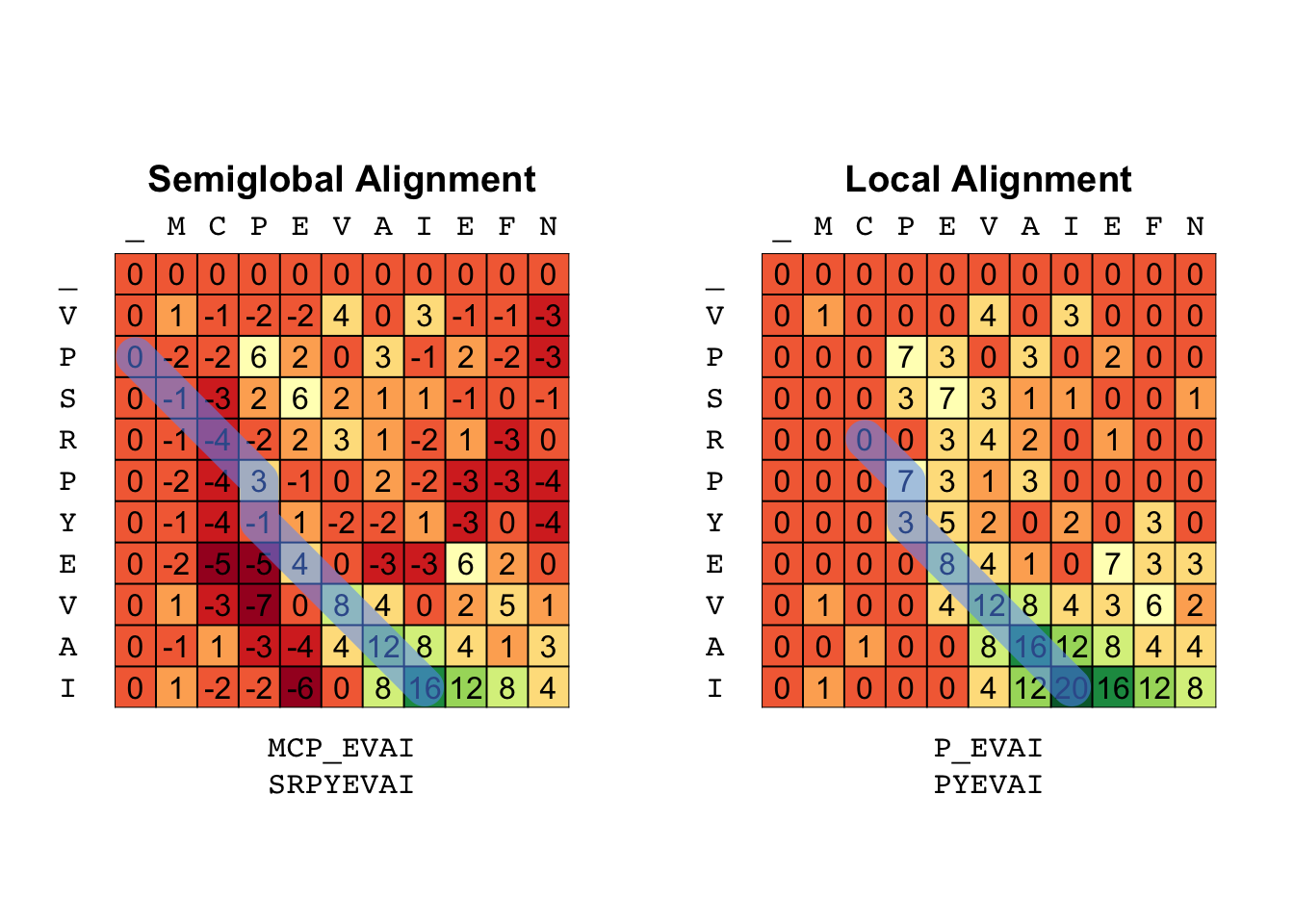
And below a simple example to illustrate the difference with the semi-global alignment

X <- "VPSRPYEVAI"
Y <- "MCPEVAIEFN"
Semi <- align(X, Y, BLOSUM62, gap = -4, type = "semi")
Local <- align(X, Y, BLOSUM62, gap = -4, type = "local")

par(mfrow = c(1, 2))
breaks <- range(c(Semi$S, Local$S))
breaks <- seq(breaks[1], breaks[2], length.out = 12)
with(Semi, plot_tableau(S, backtrack(S, P, type = "semi"), breaks = breaks))
title("Semiglobal Alignment")
with(Local, plot_tableau(S, backtrack(S, P, type = "local"), breaks = breaks))
title("Local Alignment")

Generalized Gap

Until now, we have use a homogeneous gap penalty. We could easily use different gap penalty for inserting a gap at different amino-acid without any significant change to the algorithms. A change like the following would suffice:

# Assume a vector `Gap` labeled by the different amino-acids 
Insertion <- S[i, j+1] + Gap[X[i]]
Deletion <- S[i+1, j] + Gap[Y[j]]

Another useful modification is to generalize the gap penalty even further and penalize according to its total length. With the current (homogeneous) approach, we have practically implemented a linear gap penalty function. Theory tells us that this function should be convex, ie few longer gaps should cost less than many smaller ones (for equal total length).

In either case, a significant algorithmic change is required because we now have to test every possible gap length before we decide which is the optimal alignment like:

$$ S_{i,j} = \begin{cases} S_{i-1,j-1} &+& G(x_i,y_j) \ S_{i-1,j} &+& gap(1) \ &…& \ S_{0, j} &+& gap(i) \ S_{i,j-1} &+& gap(1) \ &…& \ S_{i,0} &+& gap(j)\end{cases}$$

The most common choice, for a gap function is the affine gap penalty which is both simple and approximates a convex function. The main idea is to differentiate the cost of opening a gap form the cost of extending it. This in turn allows us to set a high “premium” for every gap opening. The formula of the affine gap penalty is:

$$ gap(n) = -g_o - g_e(n-1)$$

where \(g_o\) is the cost of opening a gap and \(g_e\) is the cost of extending it by 1.

A simple implementation of this idea is shown in the code below:

align <- function(X, Y, G, gapOpen, gapExtend, type="global") {
    ## Prepare Input
    n <- nchar(X)
    m <- nchar(Y)
    X <- unlist(strsplit(X, ""))
    Y <- unlist(strsplit(Y, ""))
    sub2ind <- function(r, c) (c-1) * nrow(S) + r

    ## Initialize Matrices
    S <- matrix(0, nrow = n+1, ncol = m+1)  # matrix full of zeros
    rownames(S) <- c("_", X)
    colnames(S) <- c("_", Y)
    P <- S
    
    ## Initialize 1st row/col
    if (type == "global") {
        S[,1] <- 0:n * gapExtend
        S[1,] <- 0:m * gapExtend
        P[,1] <- 0:n
        P[1,2:ncol(S)] <- 0:(m-1) * nrow(S) + 1
    }
    # For local alignment
    lb <- ifelse(type == "local", 0, -Inf)

    for (i in 1:n) {
        for (j in 1:m) {
            # Find where is the optimal gap opening
            Insertion <- S[i:1, j+1] + gapOpen + 0:(i-1) * gapExtend
            Deletion  <- S[i+1, j:1] + gapOpen + 0:(j-1) * gapExtend
            max_ins <- which.max(Insertion)
            max_del <- which.max(Deletion)
            # Candidate predecesors
            Candidates <- c(
                Match = S[i,j] + G[X[i], Y[j]],
                Insertion = Insertion[max_ins],
                Deletion = Deletion[max_del],
                lb = lb  # test with the lower bound
            )
            
            # if lb is the max then we set predecesor to 0
            predecesor <- list(r = c(i, i + 1 - max_ins, i+1, 0),
                               c = c(j, j+1, j + 1 - max_del, 1))
            
            imax <- which.max(Candidates)
            S[i+1,j+1] <- Candidates[imax]
            P[i+1,j+1] <- with(predecesor, sub2ind(r[imax], c[imax]))
        }
    }
    return(list(S = S, P = P))
}

The trackback function does not need any change (courtesy of our good design patter!).

As usual, below is an example illustrating the different results

X <- "YAWHEAE"
Y <- "HEAGAWGHEE"
# Global Alignment for both
LinGap <- align(X, Y, BLOSUM62, gapOpen = -4, gapExtend = -4)
AffGap <- align(X, Y, BLOSUM62, gapOpen = -12, gapExtend = -4)

par(mfrow = c(1, 2))
breaks <- range(c(LinGap$S, AffGap$S))
breaks <- seq(breaks[1], breaks[2], length.out = 12)
with(LinGap, plot_tableau(S, backtrack(S, P), breaks = breaks))
title("Linear Gap Penalty")
with(AffGap, plot_tableau(S, backtrack(S, P), breaks = breaks))
title("Affine Gap Penalty")

Affine Gap in \(O(mn)\) time - (Optional)

As you may have notice, all the algorithms so far (global, semi-global and local) required constant time per loop (some simple look ups, additions and comparisons) so their overall complexity is \(O(mn)\) time. On the other hand, the addition of affine-gaps does not require merely a change of initial of terminating conditions, it requires extra work per loop. In particular, we have to loop once more across the matrix to search where the gap opened for the first time so overall our implementation requires \(O(mn^2)\) time with \(n>m\).

However, this is only due to our “naive” (but hopefully educational) implementation. The problem can still be solve at \(O(mn)\) time at the expense of some memory. The key observation, is the optimal gap-cost is changing in a predictable way from row to row and column to column. In particular, there are to scenarios:

1. The algorithm decides to open a new gap, in which case it pays the appropriate opening penalty
2. The algorithm extends and already opened gap, in which case it only pays the regular gap penalty.

In the first case is practically the same as the case of constant gap, the only change being the cost, so we have to take it into account. The question now is, do we have to deal with each gap extension separately? Or in other words, does the optimal position to open a gap changes when we extend the gap? The answer is unsurprisingly negative, if at a previous step we found that opening a gap at position \(k\) is better than opening a gap at any other position across the row/column, then extending the gap adds a constant term to all these cost and it won't affect their ordering. So we just have to remember where was the optimal gap opening and extend it by 1.

Below we presented again the algorithm for generalize gap but we add 2 extra matrices H and V to keep track of the optimal gap opening with respect to the horizontal and vertical direction. At every iteration, we check whether it is best to open a new gap (and pay gapOpen) or extend the previous optimal gap (and pay gapExtend).

fastalign <- function(X, Y, G, gapOpen, gapExtend, type="global") {
    ## Prepare Input
    n <- nchar(X)
    m <- nchar(Y)
    X <- unlist(strsplit(X, ""))
    Y <- unlist(strsplit(Y, ""))
    sub2ind <- function(r, c) (c-1) * nrow(S) + r

    ## Initialize Matrices
    S <- matrix(0, nrow = n+1, ncol = m+1)  # matrix full of zeros
    rownames(S) <- c("_", X)
    colnames(S) <- c("_", Y)
    P <- S
    
    ## Select Type    
    if (type == "global") {
        S[,1] <- 0:n * gapExtend
        S[1,] <- 0:m * gapExtend
        P[,1] <- 0:n
        P[1,2:ncol(S)] <- 0:(m-1) * nrow(S) + 1
    }
    lb <- ifelse(type == "local", 0, -Inf)
    
    #### Difference from "naive" approach ####
    H <- V <- S  # Two new matrices to hold the optimal gap
    PH <- PV <- 1  # Positions of the optimal gap openings
    ##########################################
    
    # Main loop
    for (i in 1:n) {
        for (j in 1:m) {
            #### Check Optimal Gap position ####
            
            # Check optimal horizontal gap
            new_gap <- S[i, j+1] + gapOpen
            old_gap <- H[i, j+1] + gapExtend
            if ( new_gap > old_gap ) {
                H[i+1, j+1] <- new_gap
                PH <- i  # new position of optimal gap
            } else {
                 H[i+1, j+1] <- old_gap
                 # PH stays the same
            }
            # Check optimal vertical gap
            new_gap <- S[i+1, j] + gapOpen
            old_gap <- V[i+1, j] + gapExtend
            if ( new_gap > old_gap ) {
                V[i+1, j+1] <- new_gap
                PV <- j  # new position of optimal gap
            } else {
                V[i+1, j+1] <- old_gap
                # PV stays the same
            }
            ##################################
            
            # Compare all candidates
            Candidates <- c(
                Match = S[i,j] + G[X[i], Y[j]],
                Insertion = H[i+1, j+1],
                Deletion = V[i+1, j+1],
                Restart = lb
            )
            predecesor <- list(r = c(i, PH, i+1, 0),
                               c = c(j, j+1, PV, 1))
            
            imax <- which.max(Candidates)
            S[i+1,j+1] <- Candidates[imax]
            P[i+1,j+1] <- with(predecesor, sub2ind(r[imax], c[imax]))
            
        }
    }
    return(list(S = S, P = P))
}

Below is a small demonstration of the speed boost:

library(microbenchmark)

X <- paste(sample(Aminos, 30, replace = TRUE), collapse = "")
Y <- paste(sample(Aminos, 50, replace = TRUE), collapse = "")

microbenchmark(
    align(X, Y, BLOSUM62, -12, -4),
    fastalign(X, Y, BLOSUM62, -12, -4)
)

## Unit: milliseconds
##                                expr       min       lq     mean   median
##      align(X, Y, BLOSUM62, -12, -4) 107.92895 189.4232 244.9917 218.8904
##  fastalign(X, Y, BLOSUM62, -12, -4)  59.21983 109.9211 147.2817 127.0678
##        uq      max neval cld
##  274.3091 687.5976   100   b
##  153.9669 411.9534   100  a